lineare Gleichungssysteme

Additionsverfahren

Lisa von OnMathe
two students high five

Einleitung

Mit dem Additionsverfahren löst du ein lineares Gleichungssystem, indem du eine Variable so „wegaddierst“, dass am Ende nur noch eine übrig bleibt.

Wir starten sofort mit einem Beispiel:
\( \textsf{I. } \ \ 2{\textcolor{orange}{x}} + 3{\textcolor{green}{y}} = 12 \)
\( \textsf{II. } \ \ 4{\textcolor{orange}{x}} - 3{\textcolor{green}{y}} = 6 \)
1. Schritt: Addieren → \( {\textcolor{green}{y}} \) hebt sich auf.
\( \begin{array}{rcrccr} 2{\textcolor{orange}{x}} & + & 3{\textcolor{green}{y}} & = & 12 \\ {+} & & {+} & & {+} \\ 4{\textcolor{orange}{x}} & - & 3{\textcolor{green}{y}} & = & 6 \\ \hline 6{\textcolor{orange}{x}} & & 0 & = & 18 \end{array} \)
\(x\) berechnen:
\( 6{\textcolor{orange}{x}} = 18 \hspace{1cm} |:6 \)
\( {\textcolor{orange}{x}} = {\textcolor{orange}{3}} \)
2. Schritt: \( {\textcolor{orange}{x=3}} \) einsetzen (z. B. in Gleichung I).
\( 2{\textcolor{orange}{x}} + 3{\textcolor{green}{y}} = 12 \)
\( 2\cdot{\textcolor{orange}{3}} + 3{\textcolor{green}{y}} = 12 \)
\( 6 + 3{\textcolor{green}{y}} = 12 \hspace{1cm} |-6 \)
\( 3{\textcolor{green}{y}} = 6 \hspace{1cm} |:3 \)
\( {\textcolor{green}{y}} = {\textcolor{green}{2}} \)
3. Schritt: Lösung als Punkt notieren.
\( \textsf{L}\big({\textcolor{orange}{3}} \mid {\textcolor{green}{2}}\big) \)

Eine Variable verschwindet, die andere lässt sich lösen – so einfach ist das Prinzip.
Im Beitrag lernst du auch den Fall kennen, in dem man vorher multiplizieren muss, und kannst das Ganze mit Übungsaufgaben festigen.

Merke
1. Eine Variable durch addieren verschwinden lassen
2. Die verbleibende Variable berechnen
3. Wert einsetzen → zweite Variable bestimmen

Beispiel 1: Schritt für Schritt

Wir lösen ein lineares Gleichungssystem mit dem Additionsverfahren.
Ziel: Eine Variable soll beim Addieren oder Subtrahieren verschwinden.

\( \textsf{I. } \ \ 2{\textcolor{orange}{x}} + {\textcolor{green}{y}} = 7 \)
\( \textsf{II. } \ \ 3{\textcolor{orange}{x}} - {\textcolor{green}{y}} = 3 \)

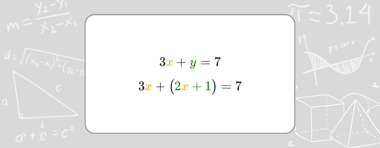
In I steht \( +y \), in II steht \( -y \). Beim Addieren hebt sich \( {\textcolor{green}{y}} \) direkt auf.

1. Schritt: Gleichung I und II addieren.
\[ \begin{array}{rcrccr} 2{\textcolor{orange}{x}} & & {\textcolor{green}{y}} & & = & 7 \\ {+} & & {+} & & & {+} \\ 3{\textcolor{orange}{x}} & & -{\textcolor{green}{y}}& & = & 3 \\ \hline 5{\textcolor{orange}{x}} & & 0 & & = & 10 \end{array} \]

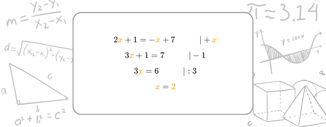
Jetzt ist \( {\textcolor{green}{y}} \) weg – übrig bleibt nur noch \( {\textcolor{orange}{x}} \).

\( 5{\textcolor{orange}{x}} = 10 \hspace{1cm} |:5 \)
\( {\textcolor{orange}{x}} = {\textcolor{orange}{2}} \)
2. Schritt: \( {\textcolor{orange}{x}} \) einsetzen, um \( {\textcolor{green}{y}} \) zu finden.
\( 2{\textcolor{orange}{x}} + {\textcolor{green}{y}} = 7 \)
\( 2\cdot{\textcolor{orange}{2}} + {\textcolor{green}{y}} = 7 \)
\( 4 + {\textcolor{green}{y}} = 7 \hspace{1cm} |-4 \)
\( {\textcolor{green}{y}} = {\textcolor{green}{3}} \)
3. Schritt: Lösung als Punkt notieren.
\( \textsf{L}\big({\textcolor{orange}{2}} \mid {\textcolor{green}{3}}\big) \)

Ergebnis: Die beiden Geraden schneiden sich in \( \big({\textcolor{orange}{2}} \mid {\textcolor{green}{3}}\big) \).

Wichtig
Es ist egal, ob du \(x\) oder \(y\) eliminierst.
Hauptsache: eine Variable fällt weg – dann kannst du die andere berechnen.
Merke
1) Eine Variable weg bekommen (addieren/subtrahieren oder vorher multiplizieren)
2) Übrig gebliebene Variable lösen
3) Wert einsetzen → zweite Variable
4) Lösung als Punkt: \( \big(x \mid y\big) \)

Beispiel 2: Gleichung umstellen

Beim Additionsverfahren werden die Gleichungen so vorbereitet, dass sich beim Addieren oder Subtrahieren eine Variable aufhebt.

Wichtig
Es ist egal, ob du \(x\) oder \(y\) eliminierst.
Hauptsache: eine Variable fällt weg – dann kannst du die andere berechnen.

Schauen wir uns das direkt an einem Beispiel an.

\( \textsf{I. } \ \ 2{\textcolor{orange}{x}} + {\textcolor{green}{y}} = {\textcolor{midnightblue}{7}} \)
\( \textsf{II. } \ \ 3{\textcolor{orange}{x}} - 2{\textcolor{green}{y}} = {\textcolor{midnightblue}{4}} \)

So wie die Gleichungen hier stehen, würde beim Addieren keine Variable verschwinden. Also machen wir sie erst „additionsbereit“.

Wir wollen \( {\textcolor{green}{y}} \) eliminieren. Dazu multiplizieren wir Gleichung I vollständig mit 2.
\[ \begin{array}{rcrccrc} 2{\textcolor{orange}{x}} & + & {\textcolor{green}{y}} & & = & {\textcolor{midnightblue}{7}} & \big|\,{\textcolor{orangered}{\cdot 2}} \\ {\textcolor{orangered}{\cdot 2}} & & {\textcolor{orangered}{\cdot 2}} & & & {\textcolor{orangered}{\cdot 2}} & \\ 4{\textcolor{orange}{x}} & + & 2{\textcolor{green}{y}} & & = & {\textcolor{midnightblue}{14}} & \end{array} \]
Merke
Beim Multiplizieren gilt: jeder Term wird mitmultipliziert – links und rechts vom „=“.

Jetzt können wir die beiden Gleichungen addieren.

\[ \begin{array}{rcrccr} 4{\textcolor{orange}{x}} & & 2{\textcolor{green}{y}} & & = & {\textcolor{midnightblue}{14}} \\ {+} & & {+} & & & {+} \\ 3{\textcolor{orange}{x}} & & -2{\textcolor{green}{y}}& & = & {\textcolor{midnightblue}{4}} \\ \hline 7{\textcolor{orange}{x}} & & 0 & & = & {\textcolor{midnightblue}{18}} \end{array} \]

Nice: Das \( {\textcolor{green}{y}} \) ist weg. Jetzt lösen wir nach \( {\textcolor{orange}{x}} \) auf.

\( 7{\textcolor{orange}{x}} = {\textcolor{midnightblue}{18}} \hspace{1cm} |:7 \)
\( {\textcolor{orange}{x}} = {\textcolor{orange}{\dfrac{18}{7}}} \)
Und jetzt kommt der Standard-Schritt: einsetzen, damit du \( {\textcolor{green}{y}} \) bekommst. Wir nehmen Gleichung I.
\( 2{\textcolor{orange}{x}} + {\textcolor{green}{y}} = {\textcolor{midnightblue}{7}} \)
\( 2\cdot{\textcolor{orange}{\dfrac{18}{7}}} + {\textcolor{green}{y}} = {\textcolor{midnightblue}{7}} \)
\( {\textcolor{midnightblue}{\dfrac{36}{7}}} + {\textcolor{green}{y}} = {\textcolor{midnightblue}{7}} \hspace{1cm} | -{\textcolor{orangered}{\dfrac{36}{7}}} \)
\( {\textcolor{green}{y}} = {\textcolor{green}{\dfrac{13}{7}}} \)

Damit kennen wir beide Variablen.

\( {\textcolor{orange}{x}} = {\textcolor{orange}{\dfrac{18}{7}}} \)
\( {\textcolor{green}{y}} = {\textcolor{green}{\dfrac{13}{7}}} \)
Zum Schluss schreiben wir die Lösung als Punkt.
\( \textsf{L}\!\left({\textcolor{orange}{\dfrac{18}{7}}} \mid {\textcolor{green}{\dfrac{13}{7}}}\right) \)
Merke
• Beim Multiplizieren immer alle Terme mitnehmen (links und rechts vom „=“).
• Eine Variable fällt nur weg, wenn die Vorzeichen gegensätzlich sind.
• Die Lösung am Ende immer als Punkt notieren: \((x \mid y)\).

Textaufgaben lösen

In Anwendungsaufgaben stellst du mit dem Text zuerst die passenden Gleichungen auf – dann berechnest du die Lösungen mit dem LGS.

Auf einem Bauernhof leben Hühner und Schweine.
Insgesamt sind es 30 Tiere.
Zählt man alle Beine zusammen, so sind es 84 Beine.
Wie viele Hühner und wie viele Schweine gibt es?

Zuerst sammeln wir die wichtigen Informationen aus dem Text.

Anzahl Tiere: 30
Anzahl Beine: 84
Huhn: 2 Beine
Schwein: 4 Beine

Jetzt legen wir fest, wofür unsere Variablen stehen.

\( {\textcolor{orange}{x}} = \) Anzahl Hühner
\( {\textcolor{green}{y}} = \) Anzahl Schweine

Aus dem Text formulieren wir nun die Gleichungen. Zuerst noch in Worten – das hilft beim Überblick.

\( \textsf{I.}\; \textsf{Anzahl Tiere} \)
\( = \textsf{Anzahl } {\textcolor{orange}{\textsf{Hühner}}} + \textsf{Anzahl } {\textcolor{green}{\textsf{Schweine}}} \)
\( \textsf{II.}\; \textsf{Anzahl Beine} \)
\( = {\textcolor{orange}{\textsf{2} \cdot \textsf{(Hühner)}}} + {\textcolor{green}{\textsf{4} \cdot \textsf{(Schweine)}}} \)

Mit unseren Variablen entsteht daraus das Gleichungssystem.

\( \textsf{I. } \ {\textcolor{orange}{x}} + {\textcolor{green}{y}} = 30 \)
\( \textsf{II. } \ 2{\textcolor{orange}{x}} + 4{\textcolor{green}{y}} = 84 \)

Wir möchten jetzt \( {\textcolor{orange}{x}} \) eliminieren, damit nur noch \( {\textcolor{green}{y}} \) übrig bleibt. Dafür multiplizieren wir die gesamte Gleichung I mit –2.

\[ \begin{array}{rcrcrc} {\textcolor{orange}{x}} & + & {\textcolor{green}{y}} & = & 30 & \big|\,{\textcolor{orangered}{\cdot(-2)}} \\ {\textcolor{orangered}{\cdot(-2)}} & & {\textcolor{orangered}{\cdot(-2)}} & & {\textcolor{orangered}{\cdot(-2)}} & \\ -2{\textcolor{orange}{x}} & - & 2{\textcolor{green}{y}} & = & -60 & \end{array} \]

Jetzt addieren wir die beiden Gleichungen.

\[ \begin{array}{rcrcr} -2{\textcolor{orange}{x}} & - & 2{\textcolor{green}{y}} & = & -60 \\ + & & + & & + \\ 2{\textcolor{orange}{x}} & + & 4{\textcolor{green}{y}} & = & 84 \\ \hline 0 & + & 2{\textcolor{green}{y}} & = & 24 \end{array} \]

Übrig bleibt nur noch \( {\textcolor{green}{y}} \).

\( 2{\textcolor{green}{y}} = 24 \)
\( {\textcolor{green}{y}} = 12 \)

Zum Schluss setzen wir \( {\textcolor{green}{y}} = 12 \) in Gleichung I ein, um \( {\textcolor{orange}{x}} \) zu berechnen.

\( {\textcolor{orange}{x}} + {\textcolor{green}{y}} = 30 \)
\( {\textcolor{orange}{x}} + 12 = 30 \hspace{1cm} \big|\,{\textcolor{orangered}{-12}} \)
\( {\textcolor{orange}{x}} = 18 \)

\( {\textcolor{orange}{x}} \) steht für die Hühner, \( {\textcolor{green}{y}} \) für die Schweine.

Auf dem Bauernhof gibt es \( {\textcolor{orange}{18}} \) Hühner und \( {\textcolor{green}{12}} \) Schweine.
Merke
• Text lesen → Infos sammeln
• Variablen festlegen und Gleichungen aufstellen
• Additionsverfahren anwenden
• Ergebnis als Antwort formulieren

Du suchst Profi-Nachhilfe mit echtem Impact? Dann bist du bei OnMathe genau richtig!

Verstehe Mathe ab der ersten Stunde.

Student lernt draußen im freien mit Notebook

Teste dein Wissen

Übungen

Löse mit dem Additionsverfahren

\( \textsf{I. } \ \ 2{\textcolor{orange}{x}} + {\textcolor{green}{y}} = 6 \)
\( \textsf{II. } \ \ 3{\textcolor{orange}{x}} - {\textcolor{green}{y}} = 9 \)

Lösung

Schritt 1: Addiere beide Gleichungen.

\( (2{\textcolor{orange}{x}} + {\textcolor{green}{y}}) + (3{\textcolor{orange}{x}} - {\textcolor{green}{y}}) = 6 + 9 \)
\( 5{\textcolor{orange}{x}} = 15 \hspace{1cm} |:5 \)
\( {\textcolor{orange}{x}} = {\textcolor{orange}{3}} \)

Schritt 2: Setze \(x = 3\) in I ein.

\( 2\cdot 3 + {\textcolor{green}{y}} = 6 \)
\( 6 + {\textcolor{green}{y}} = 6 \hspace{1cm} |-6 \)
\( {\textcolor{green}{y}} = 0 \)
Lösung: \( \textsf{L}(3 \mid 0) \)

\( \textsf{I. } \ \ 2{\textcolor{orange}{x}} + {\textcolor{green}{y}} = 7 \)
\( \textsf{II. } \ \ 3{\textcolor{orange}{x}} - 2{\textcolor{green}{y}} = 4 \)

Lösung

Schritt 1: Multipliziere I mit 2, damit sich \(y\) aufhebt.

\( 2{\textcolor{orange}{x}} + {\textcolor{green}{y}} = 7 \hspace{1cm} |\cdot 2 \)
\( 4{\textcolor{orange}{x}} + 2{\textcolor{green}{y}} = 14 \)

Schritt 2: Addiere die beiden Gleichungen.

\[ \begin{array}{rcrccr} 4{\textcolor{orange}{x}} & + & 2{\textcolor{green}{y}} & = & 14 \\ + & & + & & + \\ 3{\textcolor{orange}{x}} & - & 2{\textcolor{green}{y}} & = & 4 \\ \hline 7{\textcolor{orange}{x}} & & 0 & = & 18 \end{array} \]
\( 7{\textcolor{orange}{x}} = 18 \hspace{1cm} |:7 \)
\( {\textcolor{orange}{x}} = {\textcolor{orange}{\dfrac{18}{7}}} \)

Schritt 3: Setze \(x = \dfrac{18}{7}\) in I ein.

\( 2\cdot\dfrac{18}{7} + {\textcolor{green}{y}} = 7 \)
\( \dfrac{36}{7} + {\textcolor{green}{y}} = 7 \hspace{1cm} -\dfrac{36}{7} \)
\( {\textcolor{green}{y}} = \dfrac{13}{7} \)
Lösung: \( \textsf{L}\!\big(\tfrac{18}{7} \mid \tfrac{13}{7}\big) \)

Textaufgabe:
In einer Schule gibt es 26 Schüler, die entweder im Fußballverein oder im Basketballverein sind.
Zusammen zahlen sie Vereinsbeiträge in Höhe von 88 €.
Ein Fußballer zahlt 2 €, ein Basketballer 4 €.
Bestimme die Anzahl der Fußballer und Basketballer.

Lösung

Schritt 1: Lege die Variablen fest.

\( {\textcolor{orange}{x}} = \) Anzahl Fußballer
\( {\textcolor{green}{y}} = \) Anzahl Basketballer

Schritt 2: Stelle die Gleichungen auf.

\( \textsf{I. } \ {\textcolor{orange}{x}} + {\textcolor{green}{y}} = 26 \)
\( \textsf{II. } \ 2{\textcolor{orange}{x}} + 4{\textcolor{green}{y}} = 88 \)

Schritt 3: Multipliziere Gleichung I mit –2, damit sich die \( {\textcolor{orange}{x}} \)-Terme aufheben.

\[ \begin{array}{rcrcrcl} {\textcolor{orange}{x}} & + & {\textcolor{green}{y}} & = & 26 & \big| \cdot {\textcolor{orangered}{(-2)}} \\ -2{\textcolor{orange}{x}} & - & 2{\textcolor{green}{y}} & = & -52 \\ \end{array} \]

Schritt 4: Addiere die beiden Gleichungen.

\[ \begin{array}{rcrcr} -2{\textcolor{orange}{x}} & - & 2{\textcolor{green}{y}} & = & -52 \\ + & & + & & + \\ 2{\textcolor{orange}{x}} & + & 4{\textcolor{green}{y}} & = & 88 \\ \hline 0 & + & 2{\textcolor{green}{y}} & = & 36 \end{array} \]

Schritt 5: Löse nach \(y\) auf.

\( 2{\textcolor{green}{y}} = 36 \)
\( {\textcolor{green}{y}} = 18 \)

Schritt 6: Setze \( {\textcolor{green}{y}} = 18 \) in Gleichung I ein.

\( {\textcolor{orange}{x}} + {\textcolor{green}{18}} = 26 \)
\( {\textcolor{orange}{x}} = 8 \)

Antwort:

Es gibt \( {\textcolor{orange}{8}} \) Fußballer und \( {\textcolor{green}{18}} \) Basketballer.

Ausgewählt für Dich

Empfohlene Beiträge

Mehr dazu

in unseren FAQs

Wann ist das Additionsverfahren sinnvoll?

Das Additionsverfahren eignet sich besonders dann, wenn sich eine Variable durch Addieren oder Subtrahieren leicht eliminieren lässt.
Typisch ist:
→ gleiche Variable in beiden Gleichungen
→ gleiche oder entgegengesetzte Vorzeichen

Was mache ich, wenn sich keine Variable direkt aufhebt?

Dann bereitest du die Gleichungen vor.
→ eine oder beide Gleichungen passend multiplizieren
→ Ziel: gleiche Koeffizienten vor einer Variable
Erst danach wird addiert oder subtrahiert.

Muss ich immer beide Gleichungen verändern?

Nein.
Oft reicht es, nur eine Gleichung zu multiplizieren.
Wichtig ist nur, dass danach beim Addieren eine Variable verschwindet.

Welche Fehler passieren beim Additionsverfahren am häufigsten?

Typische Fehler sind:
→ Vorzeichen werden übersehen
→ nicht alle Terme werden mitmultipliziert
→ das Ergebnis wird nicht als Punkt notiert

Muss ich das Additionsverfahren immer verwenden?

Nein.
Es gibt mehrere Lösungsverfahren.
→ Wähle immer das Verfahren,
→ das am wenigsten Umformungen braucht.

Mehr dazu

Weiterführende Informationen

Wenn nichts direkt wegfällt: Additionsverfahren vorbereiten

Oft musst du die Gleichungen zuerst sortieren oder multiplizieren, damit sich eine Variable eliminieren lässt.

\( \textsf{I.}\quad 3{\textcolor{orange}{x}} + 2{\textcolor{green}{y}} = {\textcolor{midnightblue}{7}} \)
\( \textsf{II.}\quad 4{\textcolor{green}{y}} = 2{\textcolor{orange}{x}} + {\textcolor{midnightblue}{6}} \)
Ansage: Erst bringen wir beide Gleichungen in die Form \( a{\textcolor{orange}{x}} + b{\textcolor{green}{y}} = c \).
1. Schritt: Gleichung II sortieren (alles mit \( {\textcolor{orange}{x}} \) und \( {\textcolor{green}{y}} \) links, Zahl rechts).
\( 4{\textcolor{green}{y}} = 2{\textcolor{orange}{x}} + {\textcolor{midnightblue}{6}} \hspace{1cm} \big|\, -2{\textcolor{orange}{x}} \)
\( 4{\textcolor{green}{y}} - 2{\textcolor{orange}{x}} = {\textcolor{midnightblue}{6}} \)
Gleichung sortieren (Vorzeichen mitnehmen)
\( -2{\textcolor{orange}{x}} + 4{\textcolor{green}{y}} = {\textcolor{midnightblue}{6}} \)
\( \textsf{I.}\quad -2{\textcolor{orange}{x}} + 4{\textcolor{green}{y}} = {\textcolor{midnightblue}{6}} \)
\( \textsf{II.}\quad 3{\textcolor{orange}{x}} + 2{\textcolor{green}{y}} = {\textcolor{midnightblue}{7}} \)
Jetzt bringen wir die \({\textcolor{green}{y}}\)-Terme auf die gleiche Zahl.
Gleichung II mit 2 multiplizieren:
\[ \begin{array}{rcrccr} 3{\textcolor{orange}{x}} & + & 2{\textcolor{green}{y}} & = & {\textcolor{midnightblue}{7}} \\ \big|\,{\textcolor{orangered}{\cdot 2}} & & \big|\,{\textcolor{orangered}{\cdot 2}} & & \big|\,{\textcolor{orangered}{\cdot 2}} \\ 6{\textcolor{orange}{x}} & + & 4{\textcolor{green}{y}} & = & {\textcolor{midnightblue}{14}} \end{array} \]
3. Schritt: Jetzt addieren wir Gleichung I und II → \( {\textcolor{green}{y}} \) fällt weg.
\[ \begin{array}{rcrccr} 6{\textcolor{orange}{x}} & + & 4{\textcolor{green}{y}} & & = & {\textcolor{midnightblue}{14}} \\ {+} & & {+} & & & {+} \\ 2{\textcolor{orange}{x}} & - & 4{\textcolor{green}{y}} & & = & {\textcolor{midnightblue}{-6}} \\ \hline 8{\textcolor{orange}{x}} & & 0 & & = & {\textcolor{midnightblue}{8}} \end{array} \]
4. Schritt: \( {\textcolor{orange}{x}} \) berechnen.
\( 8{\textcolor{orange}{x}} = {\textcolor{midnightblue}{8}} \hspace{1cm} |:8 \)
\( {\textcolor{orange}{x}} = {\textcolor{orange}{1}} \)
5. Schritt: \( {\textcolor{orange}{x}} = {\textcolor{orange}{1}} \) in eine Ausgangsgleichung einsetzen (z. B. in I) und \( {\textcolor{green}{y}} \) berechnen.
\( 3{\textcolor{orange}{x}} + 2{\textcolor{green}{y}} = {\textcolor{midnightblue}{7}} \)
\( 3\cdot{\textcolor{orange}{1}} + 2{\textcolor{green}{y}} = {\textcolor{midnightblue}{7}} \)
\( 3 + 2{\textcolor{green}{y}} = {\textcolor{midnightblue}{7}} \hspace{1cm} |{\textcolor{orangered}{-3}} \)
\( 2{\textcolor{green}{y}} = {\textcolor{midnightblue}{4}} \hspace{1cm} |:2 \)
\( {\textcolor{green}{y}} = {\textcolor{green}{2}} \)
Ergebnis: Lösung als Punkt notieren.
\( \textsf{L}\big({\textcolor{orange}{1}} \mid {\textcolor{green}{2}}\big) \)
Merke
Prüfungsfall (typisch): Gleichungen sind nicht vorbereitet.
1) sortieren → \( a{\textcolor{orange}{x}} + b{\textcolor{green}{y}} = c \)
2) angleichen (multiplizieren), bis eine Variable wegfällt
3) addieren / subtrahieren → eine Variable verschwindet
4) lösen und einmal einsetzen

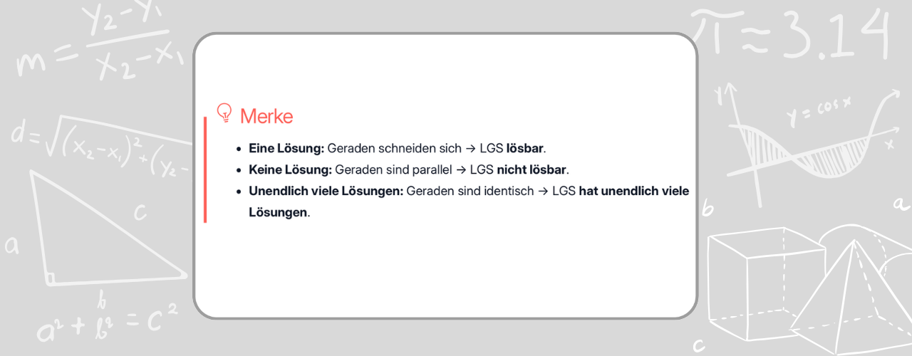
Das richtige Verfahren erkennen

In Klassenarbeiten ist entscheidend, das passende Verfahren zu erkennen. Hier siehst du kurz, wann welches Verfahren passt.

\( \textsf{I.}\quad 2{\textcolor{orange}{x}} + {\textcolor{green}{y}} = 7 \)
\( \textsf{II.}\quad 3{\textcolor{orange}{x}} - {\textcolor{green}{y}} = 3 \)
\(y\) hebt sich beim Addieren direkt auf
→ keine Umformung nötig
Additionsverfahren

Das Additionsverfahren ist besonders dann sinnvoll, wenn du eine Variable durch Addieren oder Subtrahieren schnell loswerden kannst.

Eine Variable verschwindet
→ übrig bleibt eine Gleichung mit nur einer Variable
\( \textsf{I.}\quad {\textcolor{orange}{x}} = 2{\textcolor{green}{y}} + 1 \)
\( \textsf{II.}\quad 3{\textcolor{orange}{x}} + {\textcolor{green}{y}} = 10 \)
→ \(x\) ist bereits freigestellt
→ Einsetzen geht direkt
Einsetzungsverfahren
\( \textsf{I.}\quad {\textcolor{orange}{x}} = 2{\textcolor{green}{y}} - 1 \)
\( \textsf{II.}\quad {\textcolor{orange}{x}} = -{\textcolor{green}{y}} + 5 \)
→ beide Gleichungen nach \(x\) aufgelöst
→ direkt gleichsetzen
Gleichsetzungsverfahren
Merke
Es gibt nicht das beste Verfahren.
→ Schau dir die Gleichungen an
→ entscheide, was am wenigsten Arbeit macht

Typische Fehler beim Additionsverfahren

Hier siehst du typische beim Additionsverfahren – erst falsch, dann richtig.

\( \textsf{I.}\quad {\textcolor{orange}{x}} + {\textcolor{green}{y}} = {\textcolor{midnightblue}{6}} \)
\( \textsf{II.}\quad 2{\textcolor{orange}{x}} - {\textcolor{green}{y}} = {\textcolor{midnightblue}{5}} \)
Typischer Fehler: Beim Multiplizieren wird rechts „vergessen“.
\( \textsf{I.}\quad {\textcolor{orange}{x}} + {\textcolor{green}{y}} = {\textcolor{midnightblue}{6}} \hspace{1cm} \big|\,{\textcolor{orangered}{\cdot 2}} \)
\( \textsf{I.}\quad 2{\textcolor{orange}{x}} + 2{\textcolor{green}{y}} = {\textcolor{orangered}{6}} \)
Richtig: ALLES links und rechts wird mitmultipliziert.
\( \textsf{I.}\quad {\textcolor{orange}{x}} + {\textcolor{green}{y}} = {\textcolor{midnightblue}{6}} \hspace{1cm} \big|\,{\textcolor{orangered}{\cdot 2}} \)
\( \textsf{I.}\quad 2{\textcolor{orange}{x}} + 2{\textcolor{green}{y}} = {\textcolor{midnightblue}{12}} \)
\( \textsf{I.}\quad 3{\textcolor{orange}{x}} + {\textcolor{green}{y}} = {\textcolor{midnightblue}{8}} \)
\( \textsf{II.}\quad -2{\textcolor{orange}{x}} - {\textcolor{green}{y}} = {\textcolor{midnightblue}{1}} \)
Typischer Fehler: Das Minus vor dem \(x\) wird übersehen.
\[ \begin{array}{rcrccr} 3{\textcolor{orange}{x}} & + & {\textcolor{green}{y}} & = & 8 \\ + & & + & & \\ {\textcolor{orangered}{-2}}{\textcolor{orange}{x}} & - & {\textcolor{green}{y}} & = & 1 \\ \hline {\textcolor{orangered}{5}}{\textcolor{orange}{x}} & & 0 & = & 9 \end{array} \]
Falsch gedacht: \(-2x\) wird wie \(+2x\) behandelt → Vorzeichenfehler.
Richtig: Das Minus gehört fest zum Term.
\[ \begin{array}{rcrccr} 3{\textcolor{orange}{x}} & + & {\textcolor{green}{y}} & = & 8 \\ + & & + & & \\ -2{\textcolor{orange}{x}} & - & {\textcolor{green}{y}} & = & 1 \\ \hline {\textcolor{orange}{x}} & & 0 & = & 9 \end{array} \]
\( {\textcolor{orange}{x}} = {\textcolor{midnightblue}{9}} \)
\( \textsf{I.}\quad 4{\textcolor{green}{y}} = 2{\textcolor{orange}{x}} + {\textcolor{midnightblue}{6}} \)
\( \textsf{II.}\quad 3{\textcolor{orange}{x}} + 2{\textcolor{green}{y}} = {\textcolor{midnightblue}{7}} \)
Typischer Fehler: Beim „rüberholen“ wird das Vorzeichen falsch.
\( 4{\textcolor{green}{y}} = 2{\textcolor{orange}{x}} + {\textcolor{midnightblue}{6}} \hspace{1cm} \big|\, -2{\textcolor{orange}{x}} \)
\( 4{\textcolor{green}{y}} - 2{\textcolor{orange}{x}} = {\textcolor{midnightblue}{6}} \)
\( {\textcolor{orangered}{2}}{\textcolor{orange}{x}} + 4{\textcolor{green}{y}} = {\textcolor{midnightblue}{6}} \)
Richtig: Sortieren heißt: Vorzeichen bleiben so, wie sie sind.
\( 4{\textcolor{green}{y}} = 2{\textcolor{orange}{x}} + {\textcolor{midnightblue}{6}} \hspace{1cm} \big|\, -2{\textcolor{orange}{x}} \)
\( 4{\textcolor{green}{y}} - 2{\textcolor{orange}{x}} = {\textcolor{midnightblue}{6}} \)
\( -2{\textcolor{orange}{x}} + 4{\textcolor{green}{y}} = {\textcolor{midnightblue}{6}} \)

Textaufgaben mit dem Additionsverfahren lösen

In Textaufgaben ist oft nicht das Rechnen schwer, sondern das Erkennen: Welche Infos gehören zusammen?

Ansage: Beim Additionsverfahren hast du meistens
zwei Größen (z. B. Hühner und Ziegen)
zwei Bedingungen (z. B. Anzahl Tiere und Anzahl Beine)
Auf einem Bauernhof gibt es Hühner und Ziegen.
Insgesamt sind es 20 Tiere und 56 Beine.
Größe 1: Hühner
Größe 2: Ziegen
Bedingung 1: zusammen 20 Tiere
Bedingung 2: zusammen 56 Beine
Ansage: Jetzt machen wir daraus Variablen und Gleichungen.
\( {\textcolor{orange}{x}} \) = Anzahl Hühner
\( {\textcolor{green}{y}} \) = Anzahl Ziegen
\( \textsf{I.}\quad {\textcolor{orange}{x}} + {\textcolor{green}{y}} = 20 \)
\( \textsf{II.}\quad 2{\textcolor{orange}{x}} + 4{\textcolor{green}{y}} = 56 \)
→ zwei Gleichungen, zwei Unbekannte
→ eine Variable lässt sich gleich eliminieren (nach Multiplizieren)
Additionsverfahren
Noch ein typisches Beispiel:
In einem Kino wurden Erwachsenen- und Kinderkarten verkauft.
Insgesamt wurden 120 Tickets verkauft und 840 € eingenommen.
Größe 1: Erwachsenenkarten
Größe 2: Kinderkarten
Bedingung 1: zusammen 120 Tickets
Bedingung 2: zusammen 840 € Einnahmen
Ansage: Wieder setzen wir Variablen fest.
\( {\textcolor{orange}{x}} \) = Anzahl Erwachsenenkarten
\( {\textcolor{green}{y}} \) = Anzahl Kinderkarten
\( \textsf{I.}\quad {\textcolor{orange}{x}} + {\textcolor{green}{y}} = 120 \)
\( \textsf{II.}\quad 10{\textcolor{orange}{x}} + 4{\textcolor{green}{y}} = 840 \)
→ wieder zwei Gleichungen
→ eine Variable lässt sich gut eliminieren
Additionsverfahren
Merke
Typische Additionsverfahren-Textaufgaben sind
Tieraufgaben, Ticket- oder Preisaufgaben.
Immer gilt:
→ zwei Größen
→ zwei Bedingungen
→ ein Gleichungssystem

Wusstest du schon…?

Das Additionsverfahren ist deutlich älter als Schulbücher oder Taschenrechner. Schon vor mehreren hundert Jahren nutzte man es, um Rechenprobleme im Alltag und Handel zu lösen.

Typisch waren Preis-, Waren- oder Tieraufgaben: Wie viele Dinge gibt es insgesamt – und welche Eigenschaft kommt wie oft vor?

Durch Addieren lässt sich eine Größe eliminieren.
→ Eine Gleichung verschwindet.
→ Übrig bleibt eine Rechnung mit nur einer Unbekannten.

Genau deshalb war das Additionsverfahren im Handel so beliebt: Es funktioniert übersichtlich, schnell und ganz ohne komplizierte Umformungen.

Und genau deshalb taucht es bis heute so häufig in Textaufgaben, Klassenarbeiten und Prüfungen auf – oft ist es der direkteste Weg zur Lösung.